Analyze Covid19 data from the CDC
This tutorial will show how to use R to download CDC data and create a chart showing the number of Covid-19 deaths by sex for each state
Strategy:
Let’s calculate some statistics about deaths from Covid-19 based on CDC data
- Demonstrate how to get data from an internet source
- Do some data wrangling and simple statistical analysis
- Plot results
This tutorial assumes you already have R and Rstudio. If not, please start here and then come back
Get the dataset from the CDC: https://data.cdc.gov/NCHS/Provisional-COVID-19-Deaths-by-Sex-and-Age/9bhg-hcku
On the CDC page click on the EXPORT button on the top right of the page to download the csv file called ‘Provisional_COVID-19_Death_Counts_by_Sex__Age.csv’ download it to your desktop or another folder and copy the path to the clipboard
Open R studio and click on File -> New File -> Rscript
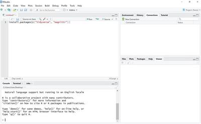
Install necessary R packages
(Why? Because you can’t load all the programs available in R - it would be way too much. You have to pick what you need and load those particular programs)
To install packages use the “install.packages()” function as shown above
or the easier way is to go to the lower right-side window of Rstudio and click on the Packages tab. Underneath, there is a button for “Install”. Click “Install” and type in the names of the packages in the pop-up box: “magrittr” , “tidyverse”. These only have to be installed once.
Load the libraries
magrittr is for piping - explained later but just so you know, the %>% in R is called a pipe. You know the picture by Rene Magritte? of the pipe? tidyverse contains many functions for data wrangling
library(magrittr)
library(tidyverse)
## -- Attaching packages --------------------------------------- tidyverse 1.3.0 --
## v ggplot2 3.3.2     v purrr   0.3.4
## v tibble  3.0.4     v dplyr   1.0.2
## v tidyr   1.1.2     v stringr 1.4.0
## v readr   1.4.0     v forcats 0.5.0
## -- Conflicts ------------------------------------------ tidyverse_conflicts() --
## x tidyr::extract()   masks magrittr::extract()
## x dplyr::filter()    masks stats::filter()
## x dplyr::lag()       masks stats::lag()
## x purrr::set_names() masks magrittr::set_names()
Load the dataset using read.csv() or read.table()
NOTE: the path to your file needs forward slashes / for R not back slashes like windows uses. If you copy your path from windows, change the slashes
Copy the path from the clipboard in the read.table() function shown below so that R knows where to find your data
covidDeaths <- read.table(file="Provisional_COVID-19_Deaths_by_Sex_and_Age.csv", sep=",", header=TRUE)
The head() function let’s you see the first few rows of data
head(covidDeaths, n=4)
##   Data.As.Of Start.Date   End.Date    Group Year Month         State       Sex
## 1 09/08/2021 01/01/2020 09/04/2021 By Total   NA    NA United States All Sexes
## 2 09/08/2021 01/01/2020 09/04/2021 By Total   NA    NA United States All Sexes
## 3 09/08/2021 01/01/2020 09/04/2021 By Total   NA    NA United States All Sexes
## 4 09/08/2021 01/01/2020 09/04/2021 By Total   NA    NA United States All Sexes
##      Age.Group COVID.19.Deaths Total.Deaths Pneumonia.Deaths
## 1     All Ages          643858      5507901           583698
## 2 Under 1 year              98        31347              336
## 3   0-17 years             412        55352              924
## 4    1-4 years              50         5798              187
##   Pneumonia.and.COVID.19.Deaths Influenza.Deaths
## 1                        320617             9272
## 2                            12               22
## 3                            93              188
## 4                            10               65
##   Pneumonia..Influenza..or.COVID.19.Deaths Footnote
## 1                                   914900
## 2                                      444
## 3                                     1431
## 4                                      292
Look at the age and sex categories
A really old and lame joke: how can you tell the difference between an epidemiologist and a clinician? The epidemiologist is broken down by age and sex
levels(as.factor(covidDeaths$Sex))
## [1] "All Sexes" "Female" "Male"
levels(as.factor(covidDeaths$Age.Group))
##  [1] "0-17 years"        "1-4 years"         "15-24 years"
##  [4] "18-29 years"       "25-34 years"       "30-39 years"
##  [7] "35-44 years"       "40-49 years"       "45-54 years"
## [10] "5-14 years"        "50-64 years"       "55-64 years"
## [13] "65-74 years"       "75-84 years"       "85 years and over"
## [16] "All Ages"          "Under 1 year"
The levels() function shows all the different categories that are included in a variable. levels only works on factors so the as.factor() function changes the character variable to a factor. How do you know if a variable is a factor or character or numeric? Look at the output from the str() function.
str(covidDeaths)
## 'data.frame':	66096 obs. of  16 variables:
##  $ Data.As.Of                              : chr  "09/08/2021" "09/08/2021" "09/08/2021" "09/08/2021" ...
##  $ Start.Date                              : chr  "01/01/2020" "01/01/2020" "01/01/2020" "01/01/2020" ...
##  $ End.Date                                : chr  "09/04/2021" "09/04/2021" "09/04/2021" "09/04/2021" ...
##  $ Group                                   : chr  "By Total" "By Total" "By Total" "By Total" ...
##  $ Year                                    : int  NA NA NA NA NA NA NA NA NA NA ...
##  $ Month                                   : int  NA NA NA NA NA NA NA NA NA NA ...
##  $ State                                   : chr  "United States" "United States" "United States" "United States" ...
##  $ Sex                                     : chr  "All Sexes" "All Sexes" "All Sexes" "All Sexes" ...
##  $ Age.Group                               : chr  "All Ages" "Under 1 year" "0-17 years" "1-4 years" ...
##  $ COVID.19.Deaths                         : int  643858 98 412 50 138 1232 3043 5395 8634 13567 ...
##  $ Total.Deaths                            : int  5507901 31347 55352 5798 9259 59389 104738 123138 150055 177545 ...
##  $ Pneumonia.Deaths                        : int  583698 336 924 187 270 1317 3071 5042 7728 11823 ...
##  $ Pneumonia.and.COVID.19.Deaths           : int  320617 12 93 10 40 496 1367 2551 4167 6714 ...
##  $ Influenza.Deaths                        : int  9272 22 188 65 80 80 148 236 324 366 ...
##  $ Pneumonia..Influenza..or.COVID.19.Deaths: int  914900 444 1431 292 448 2128 4883 8104 12494 19003 ...
##  $ Footnote                                : chr  "" "" "" "" ...
If you can see the categories above then everything seems to be working so let’s move on to data wrangling
FILTER (subset observations/rows) and SELECT (subset variables/columns)
for example, to get only the Total numbers for males and females 18-29 years and keep only the state, age group, sex, covid death numbers and total death numbers:
covidDeaths.MF.18to29 <- covidDeaths %>% filter(Group=="By Total" & Age.Group == "18-29 years" & Sex %in% (c("Male", "Female"))) %>% select(State, Age.Group, Sex, COVID.19.Deaths, Total.Deaths)
head(covidDeaths.MF.18to29)
##           State   Age.Group    Sex COVID.19.Deaths Total.Deaths
## 1 United States 18-29 years   Male            1886        76679
## 2 United States 18-29 years Female            1157        28059
## 3       Alabama 18-29 years   Male              39         1484
## 4       Alabama 18-29 years Female              22          545
## 5        Alaska 18-29 years   Male              NA          215
## 6        Alaska 18-29 years Female              NA           95
The ‘<-’ symbol is pronounced ‘gets’ and the %>% is a pipe from the magrittr package and is called ‘and then’ so the syntax in words is:
covidDeaths.MF.18to29 ‘gets’ the covidDeaths dataset ‘and then’ filters to Age.group== 18-29 and sex==Male or Female. Remember to use ‘==’ not just ‘='
Now do a little analysis:
What are the mean and median number of covid deaths across all states by male and female for 50 years and older?
- Get rid of the ‘United States’ total number and include only the state totals
- Filter to the age groups over 50: age 50-64 years, plus age 65-74 years, plus age 75-84 years, plus age 85 years and over
covidDeaths.MF.over50 <- covidDeaths %>%
  filter(Group=="By Total" & Age.Group %in% c("50-64 years", "65-74 years", "75-84 years","85 years and over") &
Sex %in% (c("Male", "Female"))) %>%
  filter(!State ==  "United States") %>%
  select(State, Age.Group, Sex, COVID.19.Deaths, Total.Deaths)
head(covidDeaths.MF.over50)
##     State         Age.Group    Sex COVID.19.Deaths Total.Deaths
## 1 Alabama       50-64 years   Male            1338        11936
## 2 Alabama       65-74 years   Male            1863        13523
## 3 Alabama       75-84 years   Male            1874        13418
## 4 Alabama 85 years and over   Male            1104         9070
## 5 Alabama       50-64 years Female            1007         7945
## 6 Alabama       65-74 years Female            1335         9984
- Calculate the mean and median number of covid deaths
covidDeaths.MF.over50 %>% group_by(Sex) %>%
  summarize(meanDeaths=mean(COVID.19.Deaths), medianDeaths=median(COVID.19.Deaths))
## `summarise()` ungrouping output (override with `.groups` argument)
## # A tibble: 2 x 3
##   Sex    meanDeaths medianDeaths
##   <chr>       <dbl>        <dbl>
## 1 Female        NA            NA
## 2 Male        1572.         1036
UGH it didn’t work! - this is because there are some states with no COVID deaths and the mean and median functions do not exclude NA values by default, i.e. median(x, na.rm = FALSE). Let’s change this function argument to TRUE so that the function will remove the NA values when computing the statistic
covidDeaths.MF.over50 %>% group_by(Sex) %>%
  summarize(meanDeaths=mean(COVID.19.Deaths, na.rm=TRUE), medianDeaths=median(COVID.19.Deaths, na.rm=TRUE))
## `summarise()` ungrouping output (override with `.groups` argument)
## # A tibble: 2 x 3
##   Sex    meanDeaths medianDeaths
##   <chr>       <dbl>        <dbl>
## 1 Female      1321.          781
## 2 Male        1572.         1036
OK first off we see clearly that the medians are smaller than the means. This tells us that there are a few states with a very high number of deaths and a bunch of other states with small numbers.
This reminds me that we should probably take into account the total number of deaths so that we can compare deaths across states while accounting for the differences in state populations.
covidDeaths.MF.over50.1 <- covidDeaths.MF.over50 %>%
  mutate(proportional.covid.deaths = ifelse(COVID.19.Deaths==0, NA, COVID.19.Deaths/Total.Deaths))
tail(covidDeaths.MF.over50.1)
##           State         Age.Group    Sex COVID.19.Deaths Total.Deaths
## 419 Puerto Rico       75-84 years   Male             396         7617
## 420 Puerto Rico 85 years and over   Male             233         6450
## 421 Puerto Rico       50-64 years Female             256         2557
## 422 Puerto Rico       65-74 years Female             269         3930
## 423 Puerto Rico       75-84 years Female             303         6491
## 424 Puerto Rico 85 years and over Female             286         9239
##     proportional.covid.deaths
## 419                0.05198897
## 420                0.03612403
## 421                0.10011732
## 422                0.06844784
## 423                0.04668002
## 424                0.03095573
covidDeaths.MF.over50.1 %>% group_by(Sex) %>%
  summarize(meanDeaths=mean(proportional.covid.deaths, na.rm=TRUE), medianDeaths=median(proportional.covid.deaths, na.rm=TRUE))
## `summarise()` ungrouping output (override with `.groups` argument)
## # A tibble: 2 x 3
##   Sex    meanDeaths medianDeaths
##   <chr>       <dbl>        <dbl>
## 1 Female      0.105        0.107
## 2 Male        0.116        0.119
That looks better - now the overall mean and median proportion of deaths due to covid19 are about the same
Look at the data. Make a graph of the proportion of covid deaths for each state by sex
Get a graphing package called ‘ggpubr’ that’s pretty easy to use. See http://www.sthda.com/english/articles/24-ggpubr-publication-ready-plots/ install the package “ggpubr” using the lower right hand box in Rstudio and then load the library using the library() function
library(ggpubr)
To plot the proportion of Covid19 deaths among people >50 by sex for each state, we have to first condense all the deaths across age groups by sex within the state because we want only 2 rows for each state; one for M and one for F because right now the data look like this:
covidDeaths.MF.over50.1 %>% select(State, Age.Group, Sex, COVID.19.Deaths, Total.Deaths, proportional.covid.deaths) %>%
head()
##     State         Age.Group    Sex COVID.19.Deaths Total.Deaths
## 1 Alabama       50-64 years   Male            1338        11936
## 2 Alabama       65-74 years   Male            1863        13523
## 3 Alabama       75-84 years   Male            1874        13418
## 4 Alabama 85 years and over   Male            1104         9070
## 5 Alabama       50-64 years Female            1007         7945
## 6 Alabama       65-74 years Female            1335         9984
##   proportional.covid.deaths
## 1                 0.1120979
## 2                 0.1377653
## 3                 0.1396631
## 4                 0.1217200
## 5                 0.1267464
## 6                 0.1337139
Here’s how to summarize (or summarise) the values within a group. Think of it as compressing multiple rows into a single summary row.
covidDeaths.StateSummary.Over50 <- covidDeaths.MF.over50.1 %>% group_by(State,Sex) %>%
      summarise(Total.DeathsOver50=sum(Total.Deaths, na.rm=TRUE),
                Total.Covid19.DeathsOver50=sum(COVID.19.Deaths, na.rm=TRUE)) %>%
  mutate(Total.prop.CovidDeathsOver50 = Total.Covid19.DeathsOver50/Total.DeathsOver50)
## `summarise()` regrouping output by 'State' (override with `.groups` argument)
head(covidDeaths.StateSummary.Over50)
## # A tibble: 6 x 5
## # Groups:   State [3]
##   State   Sex    Total.DeathsOver~ Total.Covid19.Deaths~ Total.prop.CovidDeaths~
##   <chr>   <chr>              <int>                 <int>                   <dbl>
## 1 Alabama Female             46367                  5427                  0.117
## 2 Alabama Male               47947                  6179                  0.129
## 3 Alaska  Female              2628                   148                  0.0563
## 4 Alaska  Male                3465                   230                  0.0664
## 5 Arizona Female             52854                  6500                  0.123
## 6 Arizona Male               61200                  9242                  0.151
We have the data summarized nicely so we can try plotting:
CovidStates <- ggbarplot(covidDeaths.StateSummary.Over50, x = "State", y = "Total.prop.CovidDeathsOver50",
          fill = "Sex", color = "Sex",
          palette = c("pink", "blue"),
          position = position_dodge(0.9),
          title="Proportion of total deaths due to Covid19 in people 50 and older \nby sex and state",
          x.text.angle = 90, xlab=FALSE, ylab="Proportion of Covid19 deaths"
          )
CovidStates + font("x.text", size=10)
 This chart shows that across the states the proportion of deaths due to covid19 is generally a bit higher in Males. I will look at the male/female difference in death rate in another post
HINT if the chart is squeezed into the viewer box, pull the lower right frame sideways to make it bigger
to export the plot to a file - change to your path using code like this: CovidStates %>% ggexport(width = 800, height = 500, filename = “yourpath/CovidStates.png”)
Bonnie Thiel
data scientist
My area of expertise is in applying the tools of statistics and informatics to study problems in biology and medicine.